MCCCS
Multi Channel Classification and Clustering System
This project is maintained by OpenImageAnalysisGroup
Application examples
The MCCCS contains support scripts, which process two main examples to show the capabilities of the system:- Three image sets (A1, A2, A3) from the Leaf Segmentation Challenge (LSC) 2014
- A hyperspec example from Purdue Research Foundation.
- Disease classification for detached barley leaves (in preparation, not published yet).
prepare_datasets.sh command from the terminal. The script downloads and stores the needed data and libraries using the recommended naming and folder structure. The analysis can be started by navigating into a example subfolder, here the processing script has to be executed in a terminal.
(For downloading and analyzing the application examples we include a script in the mcccs relaese, please have a look in the online documentation or in the short pdf user documentation.)
Segmentation Example
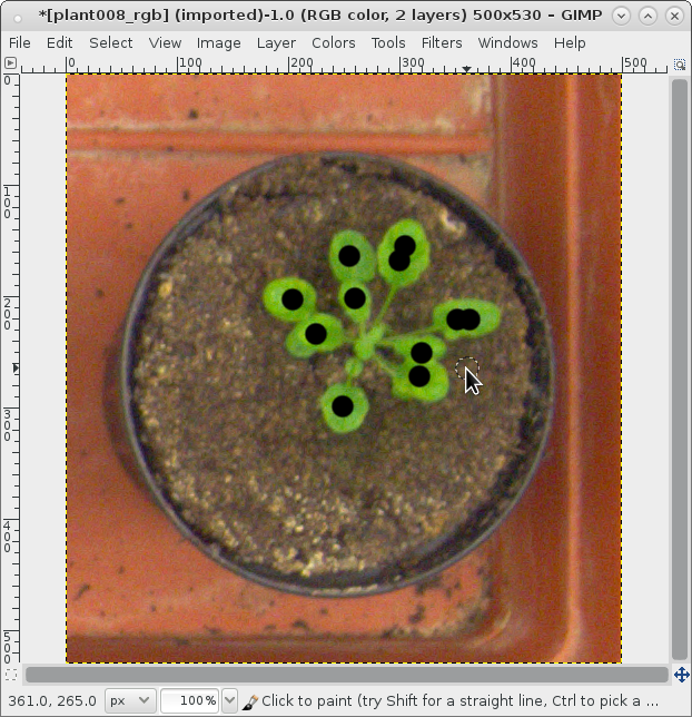
Here we show some example for foreground/background segmentation of a top-view plant image by using an supervised classifier. The first image is used as input. The second shows the creation of a foreground label which will used as training data for the classifier. It is not mandatory to label the whole image, it is sufficient to label only parts. The third image shows the classification result.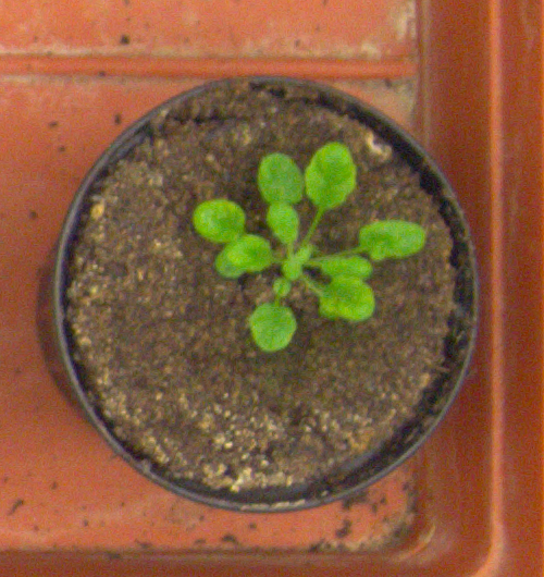 |
 |
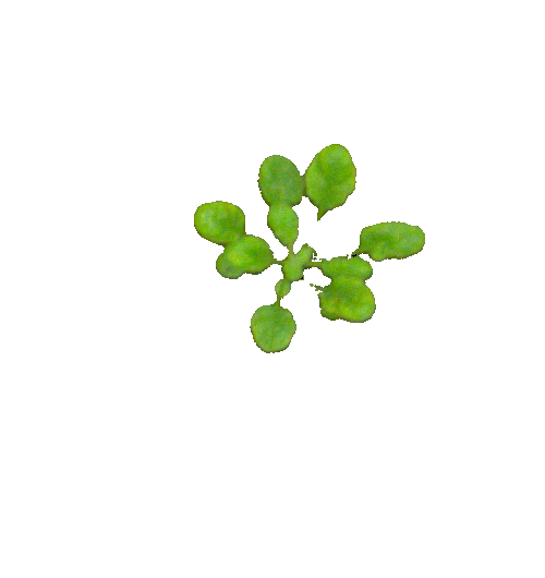 |
| Input image (source: LSC 2014) | Labeling foreground pixels (plant) during ground truth mask creation, by using gimp. | Classification result |
Results
By using a Random Forest Classifier (tree-depth 100) we gain the following qualities in case of foreground/background segmentation. Here, we use no additional image processing filters e.g. to remove noise or artifacts which could be improve the results. Especially for the A3 dataset other plant parts are in focus, these are not considered by the provided ground truth labels and counted as miss-classified. This circumstance slightly decreases the classification result.| Datasets | A1 | A2 | A3 |
| FGBGDice | 96.7 | 96.4 | 86.7 |
Classification and Clustering Example
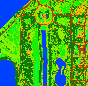
The system is also able to process hyperspectral data. Here a hyperspectral airbone data set is used to perform an un-supervised clustering and a supervised classification. The first image shows a RGB visualization (composite of 700 nm, 530 nm, 450 nm spectral bands). The second image includes the labeled classes by performing an clustering by using the EM (Expectation Maximization) algorithm. The third image shows the result of supervised classification. For this approach crude labels was prepared before and used for classifier training.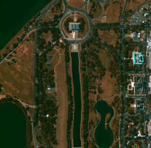 |
 |
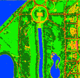 |
| RGB visualization (data source: Purdue Research Foundation) | Clustering result (using 7 classes) | Classification result (using 7 ground truth masks for training) |
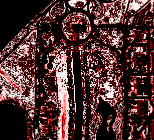
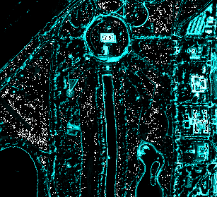
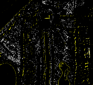
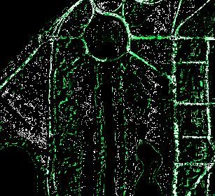
The machine learning approach generally calculates probabilities for each class. The following images visualize these probabilities for the classification (black indicates P(0), white indicates P(1)).
 |
 |
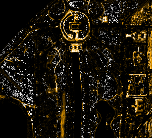 |
| Class 1 (vegetation, grass) | Class 2 (streets, trails) | Class 3 (buildings) |
 |
 |
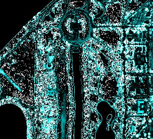 |
| Class 4 (shadows) | Class 5 (streets, trails) | Class 6 (vegetation, trees) |
 |
||
| Class 7 (water) |